Welcome To Sora Park

Both the gradient vector and Hessian matrix are used in optimisation, particularly in continuous optimisation problems.

The gradient vector is a vector of the first partial derivatives of a scalar-valued function f(x) with respect to its n variables:

$$ \bigtriangledown f(x)= { \left [ \frac{\partial f}{\partial _{x_1}}, \frac{\partial f}{\partial _{x_2}},..., \frac{\partial f}{\partial _{x_n}} \right ] }^T $$

The gradient vector is used to find the direction of steepest ascent or descent of a scalar-valued function, depending on the problem (minimisation or maximisation). Especially in machine learning, it is essential for training models via backpropagation, where it guides parameter updates to minimise loss functions.

The Hessian matrix is an n × n matrix of the second partial derivatives of the function:

$$ H_f(x) = \nabla^2 f(x) =  \frac{\partial^2 f}{\partial x_i \partial x_j} = \begin{bmatrix} \frac{\partial^2 f}{\partial x_1^2} & \frac{\partial^2 f}{\partial x_1 \partial x_2} & \cdots & \frac{\partial^2 f}{\partial x_1 \partial x_n} \\ \frac{\partial^2 f}{\partial x_2 \partial x_1} & \frac{\partial^2 f}{\partial x_2^2} & \cdots & \frac{\partial^2 f}{\partial x_2 \partial x_n} \\ \vdots & \vdots & \ddots & \vdots \\ \frac{\partial^2 f}{\partial x_n \partial x_1} & \frac{\partial^2 f}{\partial x_n \partial x_2} & \cdots & \frac{\partial^2 f}{\partial x_n^2} \end{bmatrix} $$

In optimisation, the Hessian matrix is used to determine whether a point is a local minimum, local maximum, or saddle point, and to understand the curvature of the objective function for better convergence. Methods such as Newton's method and quasi-Newton methods use the Hessian to update parameters, leveraging both first and second derivatives to find optima more efficiently than gradient-only methods.

To generalise the gradient for functions with multiple outputs, the Jacobian matrix is used. It is a matrix of all first-order partial derivatives of a vector-valued function.

A vector-valued function f(x) is defined as:

$$ f(x)=\begin{bmatrix} f_1(x_1,x_2,...,x_n) \\ f_2(x_1,x_2,...,x_n) \\ \vdots  \\ f_m(x_1,x_2,...,x_n) \end{bmatrix} $$

The Jacobian matrix of f(x) is:

$$ J_f(x) = \begin{bmatrix}
\frac{\partial f_1}{\partial x_1} & \frac{\partial f_1}{\partial x_2} &
 \cdots  & \frac{\partial f_1}{\partial x_n} \\

\frac{\partial f_2}{\partial x_1} & \frac{\partial f_2}{\partial x_2} &
 \cdots  & \frac{\partial f_2}{\partial x_n} \\

\vdots  & \vdots  & \ddots  & \vdots  \\

\frac{\partial f_m}{\partial x_1} & \frac{\partial f_m}{\partial x_2} &
 \cdots  & \frac{\partial f_m}{\partial x_n} \\
\end{bmatrix} $$

The Jacobian plays a key role in backpropagation (especially in layers with multiple outputs) in machine learning, and is also used in Newton's method for solving systems of nonlinear equations involving vector-valued functions.

SGD (Stochastic Gradient Descent) and ADAM (Adaptive Moment Estimation) are both widely used optimisation algorithms for training machine learning and deep learning models. While both use mini-batches to update parameters, Adam is an advanced adaptive optimisation algorithm, not a simple variant of SGD.

The key idea behind mini-batch SGD is to approximate the gradient of the loss function using a small, randomly selected mini-batch of data at a time, rather than the entire dataset. At each training iteration, the algorithm performs the following steps:

1. Pick a random training sample (b examples)
2. Compute the gradient of the loss function with respect to the model parameters for this sample
   $$ _{\bigtriangledown _{mini-batch}}J(_{\theta _t})=\frac{1}{b}\sum_{(x^{(j)},y^{(j)})\in B}^{}\bigtriangledown L(_{h_{_{\theta _t}}}(x^{(j)}),y^{(j)}) =_{g_t} $$
3. Update the parameters in the opposite direction of the gradient, scaled by the learning rate α to minimize the loss
   $$ _{\theta _{t+1}}=_{\theta _t}-\alpha _{\bigtriangledown _{mini-batch}}J(_{\theta _t}) $$

Adam combines the best of both SGD with momentum and adaptive learning rate methods. It maintains two exponentially decaying moving averages for each parameter:

• The gradients (the first moment, similar to momentum)
• The squared gradients (the second moment, similar to RMSprop)

The update rule for each training iteration is as follows:

1. Compute the gradient of the loss function with respect to the parameters
2. Update the biased moving average of the first moment (m) and the second moment (v)
   $$  _{m_t}={_{\beta _1}}{_{m_{t-1}}}+(1-_{\beta _1})_{g_t} $$
   $$  _{v_t}={_{\beta _2}}{_{v_{t-1}}}+(1-_{\beta _2})_{g_t^{2}} $$
   This is an exponentially decaying average of the squared gradients.
3. Compute bias-corrected estimates for both moments. This step is necessary because the moments are initialized to zero, which can bias them towards zero, especially during early training steps
   $$ _{\hat{m}_t}=\frac{_{m_t}}{1-{_{\beta _1}}^{t}} $$
   $$ _{\hat{v}_t}=\frac{_{v_t}}{1-{_{\beta _2}}^{t}} $$
4. Update the parameters using the bias-corrected moment estimates
   $$ _{\theta _{t+1}}=_{\theta _t}-\frac{\alpha }{\sqrt{_{\hat{v}_t}}+\epsilon }{_{\hat{m}_t}} $$

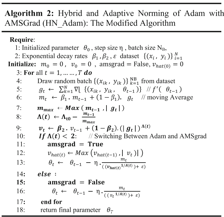
HN Adam is a modified Adam algorithm introduced by Reyad, M., Sarhan, A.M., and Arafa, M. in their 2023 paper, "A modified Adam algorithm for deep neural network optimization" [1]. The algorithm is based on a hybrid approach that combines the original Adam algorithm with the AMSGrad algorithm and incorporates an adaptive norm technique. The letters "H" and "N" in the name refer to the 'hybrid' and 'adaptive norm' components, respectively.

This algorithm's key feature is its adaptive norm technique, which adjusts the learning rate step size. According to the paper, the norm value is adaptively computed based on the maximum of the absolute value of the current gradient and the exponential moving average of past gradients. The threshold value of the norm is also randomly chosen.

The researchers found that this hybrid mechanism enhanced the generalisation performance and achieved a high speed of convergence for most deep neural network architectures.

HN Adam was selected for my final project on breast cancer detection using deep learning. The algorithm's potential to enhance the performance of a modified U-Net model was a key factor in its selection, particularly due to the need for a more dynamic learning rate strategy. This was necessary to address a challenge where the model’s evaluation metrics were stagnating around a specific value during training.

To validate the model's effectiveness, a comprehensive evaluation was conducted using both the metrics reported in the original paper and additional performance indicators, including the Dice coefficient, Jaccard index, and various confusion matrix-based metrics. Among these, the Dice coefficient and Jaccard index served as the primary evaluation criteria.

After training for 1,000 epochs, the model achieved its best performance on the validation dataset as follows:

• Dice Coefficient: 97.56%
• Jaccard Index: 95.56%
• Precision: 98%
• Recall: 97%
• F1-Measure: 98%
• Accuracy: 99.97%
• Loss: 0.033495

The project is still in progress, and additional details and final results will be shared upon completion.

Reference:

[1] Reyad, M., Sarhan, A.M. and Arafa, M. (2023). A modified Adam algorithm for deep neural network optimization. A modified Adam algorithm for deep neural network optimization.

To avoid significant noise amplification when the number of training data are small, an approach is to add an extra term (extra constraint) to the least-squares cost function.

• The extra term penalises the norm of the coefficient vector.

Modifying cost functions to favour structured solutions is called regularisation. Least-squares regression combined with l2-norm regularisaion is known as ridge regression in statistics and as Tikhonov regularisation in the literature on inverse problems.

In the simplest case, a positive multiple of the sum of squares of the variables is added to the cost function:

$$ \sum_{i=1}^{k}(a_i^Tx-b_i)^2+\rho \sum_{i=1}^{n}x_i^2 $$

where

$$ \rho>0 $$

• The extra terms result in a sensible solution in cases when minimising the first sum only does not

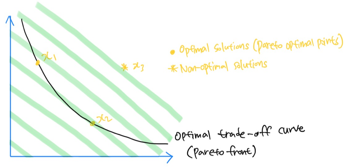
To refine the choice among Pareto optimal solutions, the objective function landscape can be adjusted by adding specific terms.

A least-squares problem is an optimisation problem with no constraints and an objective, which is as follows:

minimise

$$ f_0(x)=\left\|Ax-b \right\|_2^2=\sum_{i=1}^{k}(a_i^Tx-b_i)^2 $$

The objective function is a sum of squares of terms of the form

$$ a_i^Tx-b_i $$

The solution can be reduced to solving a set of linear equations,

$$ f(x)=\left\| Ax-b\right\|_2^2=(A_x-b)^T(Ax-b) $$

$$ =((Ax)^T-b^T)(Ax-b) $$
$$ =x^TA^TAx-b^TAx-x^TA^Tb+b^Tb $$

If x is a global minimum of the objective function, then its gradient is the zero vector.

$$ \triangledown f(x)=(\frac{\partial f}{\partial x_1},...,\frac{\partial f}{\partial x_n}) $$

The gradients are:

$$ \triangledown(x^TA^TAx)=2A^TAx, \triangledown(b^TAx)=A^Tb, \triangledown(x^TA^Tb)=A^Tb $$

Calculate these gradients with respect to

$$ x_1,...,x_n $$

Thus, the gradient of the objective function is

$$ \triangledown f(x)=2A^TAx-A^Tb-A^Tb=2A^TAx-2A^Tb $$

To find the least squares solution, we can solve

$$ \triangledown f(x)=0 $$

Or equivalently

$$ A^TAx=A^Tb $$

So we have the analytical solution:

$$ x=(A^TA)^{-1}A^Tb $$

To recognise an optimisation problem as a least-squares problem, we only need to verify that the objective is a quadratic function.