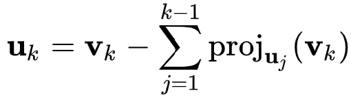
The De Moivre's formula is:
$$ [r(cos\theta + (\imath *sin\theta ))]^n=r^n((cos * n\theta) + (i * sin * n\theta)) $$
The following two terms are complex numbers, which are the combinations of a Real Number and Imaginary Number:
$$ \imath *sin\theta\ $$
$$ i * sin * n\theta $$
- A Real Number is the type of number: 1.4, 5/8, -2390, 0, for example.
- An Imaginary Number gives a negative result when squared: i^2=-1
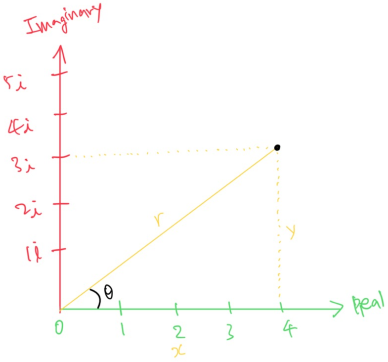
The complex number is
$$ 4 + 3\imath $$
r is
$$ r = \sqrt{4^2+3^2}=\sqrt{25}=5 $$
angle (in radian) is
$$ \Theta =tan^{-1}(y/x)=tan^{-1}(3/4)=0.6435 $$
x is
$$ cos(\theta)=x/r $$
$$ x=r*cos(\theta)=5*cos(0.6435)=4 $$
y is
$$ sin(\theta)=y/r $$
$$ y=r*sin(\theta)=5*sin(0.6435)=3 $$
Here is the common way to write the complex number below:
$$ x+(i*y)=r(cos\theta + (i*(sin\theta)))=r*cis\theta $$
- Note that a combination of cos and sin is often shortened to 'cis'
In the case, therefore, the complex number can be written as follows:
$$ 4+3i=5*cis(0.6435) $$
In the De Moivre's formula,
$$ [r(cos\theta + (\imath *sin\theta ))]^n=r^n((cos * n\theta) + (i * sin * n\theta)) $$
magnitude becomes
$$ r^n $$
angle (in radian) becomes
$$ n\theta $$
In the above case, the De Moivre formula is
$$ (5*cis(0.6435))^2=5^2*cis(2*0.6435)=25*cis(1.287) $$
So, the magnitude is 25 and the angle is 1.287 in radian.
'Mathematics' 카테고리의 다른 글
| Vector Normalisation 벡터 정규화 (0) | 2023.10.24 |
|---|---|
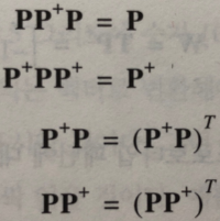
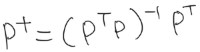
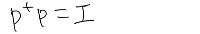
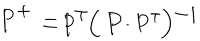
| Moore-Penrose inverse 무어-펜로즈 의사역행렬 (0) | 2023.09.13 |
| Gram-Schmidt orthogonalization (0) | 2023.07.24 |
| Pascal's rule (0) | 2021.09.02 |
| Combinations with repetition (0) | 2021.08.26 |