Welcome To Sora Park

pocketsphinx

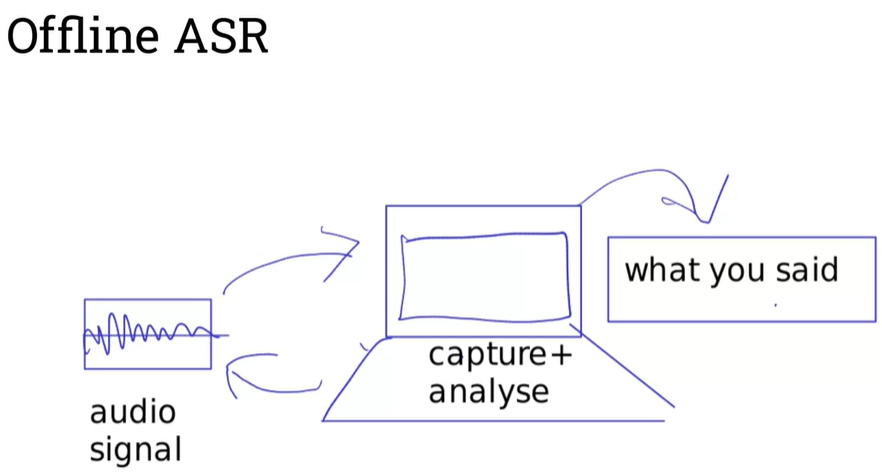
• Offline speech recognition in real-time on mobile devices, ported from the CMUSphinx project

How to use pocketsphinx:

pip install pocketsphinx

# Pocketsphinx on live input
from pocketsphinx import LiveSpeech
for phrase in LiveSpeech(): print(phrase)

# Pocketsphinx for keywords
from pocketsphinx import LiveSpeech
speech = LiveSpeech(lm=False, keyphrase='move forward', kws_threshold=le-20)
for phrase in speech: print(phrase.segments(detailed=True))

# Specify phrases in an external file
from pocketsphinx improt LiveSpeech
speech = LiveSpeech(lm=False, kws='./kws.text')
for phrase in speech: print(phrase.segments(detailed=True))
# File contents:
#	move forward /le-40/
#	go backwards /le-40/
#	turn left /le-20/
#	turn right /le-20/

# Pocketsphinx and audio files
from pocketsphinx import Pocketsphinx
ps = Pocketsphinx()
ps.decode(audio_file='nines.wav')
ps.hypothesis()
ps.confidence()
ps.best(count=4)

from pocketsphinx import Pocketsphinx
ps = Pocketsphinx(l=False, kws='./kws.txt')
ps.decode(audio_file='nines.wav')
ps.hypothesis()

vosk

• An easy to install API which is able to run efficient offline Kaldi models
• A neat wrapper around kaldi models

kaldi

• Large, open source collection of components for constructing ASR system based on finite-state transducers
  • Finite-state transducer
    : Intuitively - a simplified version of an HMM (Hidden Markov Model)
    → The tagging speed when using transducers is up to five times higher than when using the underlying HMMs. The main advantage of transforming an HMM is that the resulting transducer can be handled by finite state calculus.

Mozilla DeepSpeech

• An open source embedded (offline, on-device) speech-to-text engine which can run in real time on devices ranging from a Raspberry pi 4 to high power GPU servers

A Fourier Transform (FT) is an integral transform that takes a function as input and outputs another function that describes the extent to which various frequencies are present in the original function.

Discrete Fourier Transform (DFT)

• Since the real world deals with discrete data (samples), the DFT is a crucial tool. It's the discrete version of the FT, specifically designed to analyse finite sequences of data points like those captured by computers.
• The DFT transforms these samples into a complex-valued function of frequency called the Discrete-Time Fourier Transform (DTFT).

Discrete Cosine Transform (DCT)

• The DCT is closely related to the DFT.  While DFT uses both sines and cosines (complex functions), DCT focuses solely on cosine functions. This makes DCT computationally simpler and often preferred for tasks where the data has even symmetry (like audio signals).

Fast Fourier Transform (FFT)

• The DFT is powerful, but calculating it directly can be computationally expensive for large datasets. This is where the Fast Fourier Transform (FFT) comes in. It's a highly optimized algorithm specifically designed to compute the DFT efficiently, especially when the data length is a power of 2 (like 16, 32, 64 etc.).
• The FFT is not a theoretical transform. It is just a fast algorithm to implement the transforms when N=2^k.

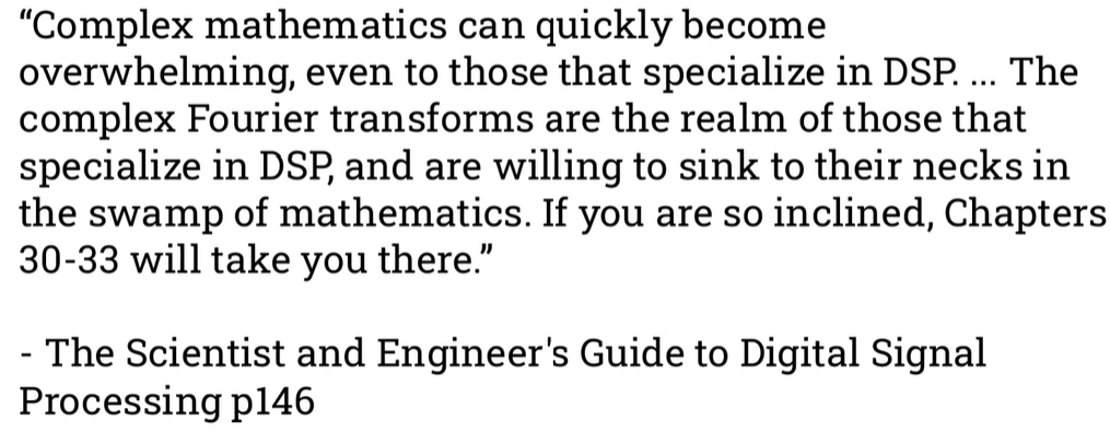
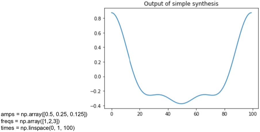
The first step is to move from simple synthesis to complex synthesis.

What's wrong with the DCT?

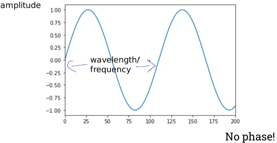
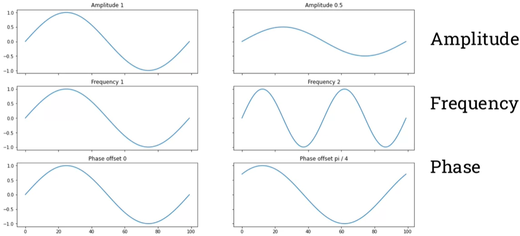
The properties of sinusoids (sine waves): frequency, phase, and amplitude

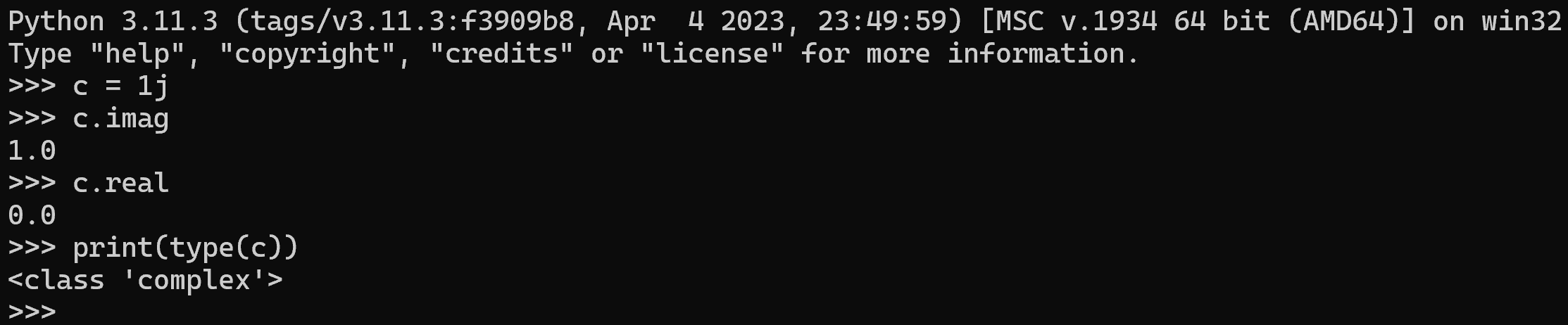
We need a way to store phase and amplitude in the same place. That is called a complex numbers.

• A complex number is basically two numbers stuck together.
  

  

  • Think of them as a way of storing phase and amplitude in one place, with associated mathematics to work with the complex numbers similarly to how we work with 'simple' numbers.
    → Complex numbers have a real and an imaginary part (two numbers).

Complex numbers in Python:

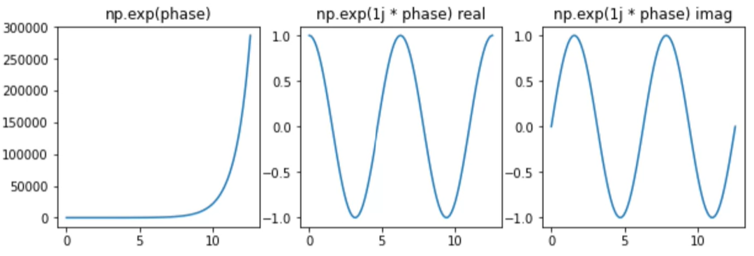
We need a way to computer waveforms from complex numbers: the exponential function

• numpy.exp(x) is the exponential function, or
• e^x (where e is Euler's number: approximately 2.718281)

→ numpy.exp(1j * x) converts x into a complex number then does exp!

Simple synthesis:

def synthesise_simple(amps, fs, ts):
    args = np.outer(ts, fs)
    M = np.cos(np.pi*2 * args)
    ys = np.dot(M, amps)
    return ys

Complex synthesis:

def synthesise_complex(amps, fs, ts):
    args = np.outer(ts, fs)
    M = np.exp(1j * np.pi*2 * args) # Swap out from np.cos(np.pi*2 * args)
    ys = np.dot(M, amps)
    return ys

The complex analysis problem:

• Given a signal and a set of frequencies, how can we find the amplitude and phase of each frequency component?

Simple analysis with numpy.linalg.solve and the DCT:

def analyse_simple(ys, fs, ts):
    args = np.outer(ts, fs)
    M = np.cos(np.pi*2 * args)
    amps = np.linalg.solve(M, ys)
    return amps
    
# More constrained version
def dct_iv(ys):
    N = len(ys)
    ts = (0.5 + np.arange(N)) / N
    fs = (0.5 + np.arange(N)) / 2
    args = np.outer(ts, fs)
    M = np.cos(np.pi*2 * args)
    amps = np.dot(M, ys) / (N / 2)
    return amps

Complex analysis with np.linalg.solve:

def analyse_complex(ys, fs, ts):
    args = np.outer(ts, fs)
    M = np.exp(1k * np.pi*2 * args)
    amps = np.linalg.solve(M, ys)
    return amps

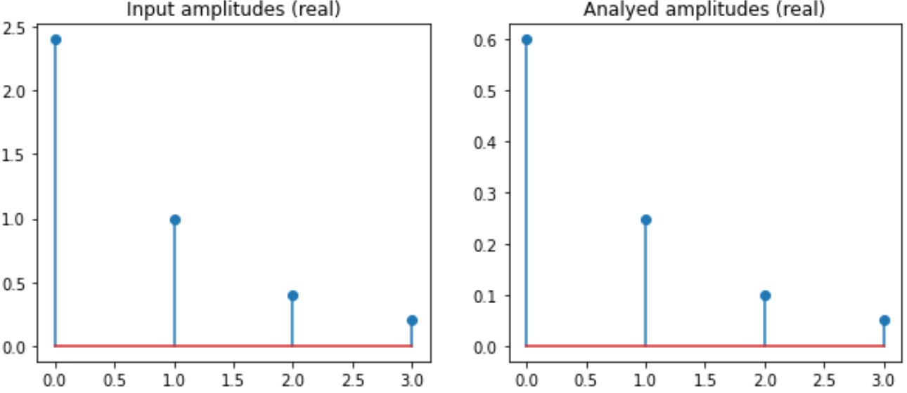
def analyse_nearly_dft(ys, fs, ts):
    N = len(fs)
    args = np.outer(ts, fs)
    M = np.exp(1j * np.pi*2 * args)
    amps = M.conj().transpose().dot(ys) / N # Swap out from 'amps = np.linalg.solve(M, ys)
    return amps

Final steps for the actual DFT:

# Calculate the frequency and time matrix
def synthesis_matrix(N):
    ts = np.arange(N) / N
    fs = np.arange(N)
    args = np.outer(ts, fs)
    M = np.exp(1j * np.pi*2 * args)
    return M
    
# Transform
def dft(ys):
    N = len(ys)
    M = synthesis_matrix(N)
    amps = M.conj().transpose().dot(ys) # No more '/ N'!
    return amps

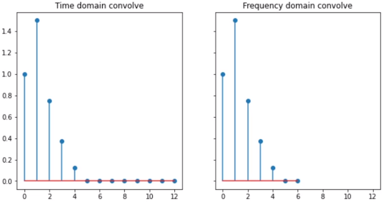
Fast convolution with the DFT

• Convolving signals in the time domain is equivalent to multiplying their Fourier transforms in frequency domain.

The inverse DFT

def idft(ys):
    N = len(ys)
    M = synthesis_matrix(N)
    amps = M.dot(ys) / N
    return amps

Signal averaging is a signal processing technique that tries to remove unwanted random disturbances from a signal through the process of averaging.

• Averaging often takes the form of summing a series of signal samples and then dividing that sum by the number of individual samples.

The following equation represents a N-point moving average filter, with input the array x and outputs the averaged array y:

$$ y(n)=\frac{1}{N}\sum_{k=0}^{N-1}x(n-k) $$

Implementing in Python:

### 1. Simple example
import numpy as np

values = np.array([3., 9., 3., 4., 5., 2., 1., 7., 9., 1., 3., 5., 4., 9., 0., 4., 2., 8., 9., 7.])
N = 3

averages = np.empty(len(values))
for i in range(1, len(values)-1):
    averages[i] = (values[i-1]+values[i]+values[i+1])/N

# Preserve the edge values
averages[0] = values[0]
averages[len(values)-1] = values[len(values)-1]

### 2. Use numpy.convolve
window = np.ones(3)
window /= sum(window)
averages = np.convolve(values, window, mode='same')

### 3. Use scipy.ndimage.uniform_filter1d
from scipy.ndimage.filters import uniform_filter1d
averages = uniform_filter1d(values, size=3)

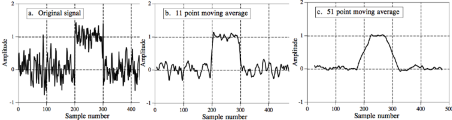
Averaging low-pass filter

In signal processing, the moving average filter can be used as a simple low-pass filter. The moving average filter smooths out a signal, removing the high frequency components from it, and this is what a low-filter does!

FIR (Finite Impulse Response) filers

In signal processing, a FIR filer is a filter whose impulse response (or response to any finite length input) is of finite duration, because it settles to zero in finite time. For a general N-tap FIR filter, the nth output is:

$$  y(n)=\sum_{k=0}^{N-1}h(k)x(n-k) $$

$$ h(n)=\frac{1}{N} $$

$$ n=0,1,...,N $$

This fomula has already been used above, since the moving average filter is a kind of FIR filter.

Implementing in Python:

import numpy as np
from thinkdsp import SquareSignal, Wave

# suppress scientific notation for small numbers
np.set_printoptions(precision=3, suppress=True)

# The wave to be filtered
from thinkdsp import read_wave
my_sound = read_wave('../Audio/429671__violinsimma__violin-carnatic-phrase-am.wav')
my_sound.make_audio()

# Make a 5-tap FIR filter using the following coefficients: 0.1, 0.2, 0.2, 0.2, 0.1
window = np.array([0.1, 0.2, 0.2, 0.2, 0.1])

# Apply the window to the signal using np.convolve
filtered = np.convolve(my_sound.ys, window, mode='same')
filtered_violin = Wave(filtered, framerate=my_sound.framerate)
filtered_violin.make_audio()

LTI (Linear Time Invariant) systems

• It it happens to be a LTI system, we can represent its behaviour as a list of numbers known as an IMPULSE RESPONSE.

An impulse response is the response of an LTI system to the impulse signal.

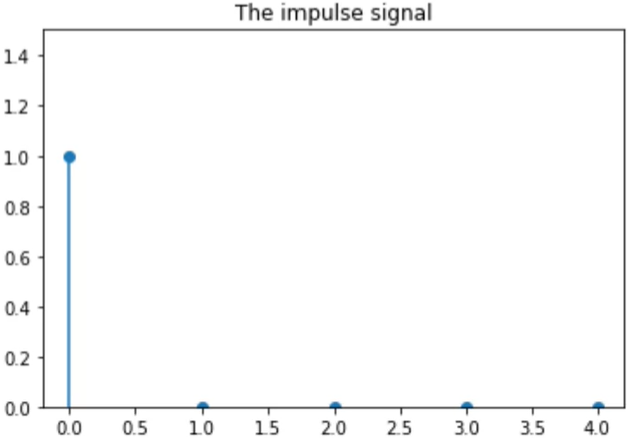
• An impulse is one single maximum amplitude sample.

Example of an impulse:

Example of an impulse response:

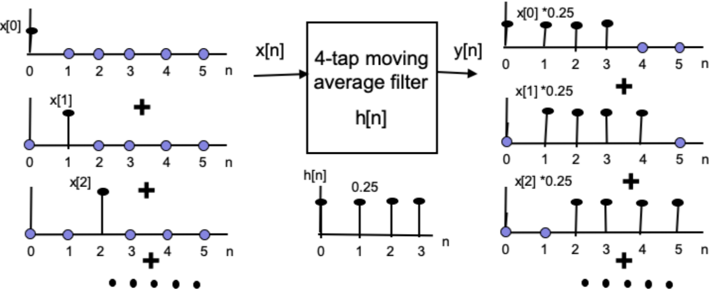
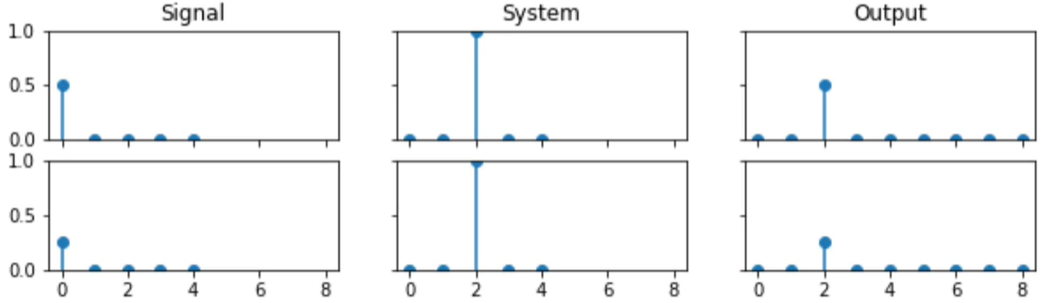
Given an impulse response, we can easily process any signal with that system using convolution.

• We can derive the output of a discrete linear system, by adding together the system's response to each input sample separately. This operation is known as convolution.

$$ y[n]=x[n]*h[n]=\sum_{m=0}^{\infty }x[m]h[n-m] $$

※ The convolution operator is indicated by the '*' operator

Three characteristics of LTI systems

Linear systems have very specific characteristics which enable us to do the convolution:

1. Homogeneity (or linear with respect to scale)
   

   

   : Multiply the signal by 0.5 (scale it by 0.5), shove both the signals through the systemsl, and get the outputs
   1) Convolve the signal with the system
   2) Receive the output
   → It doesn't matter if the signal is scaled becuse we know tht it will produce the same scaled output.
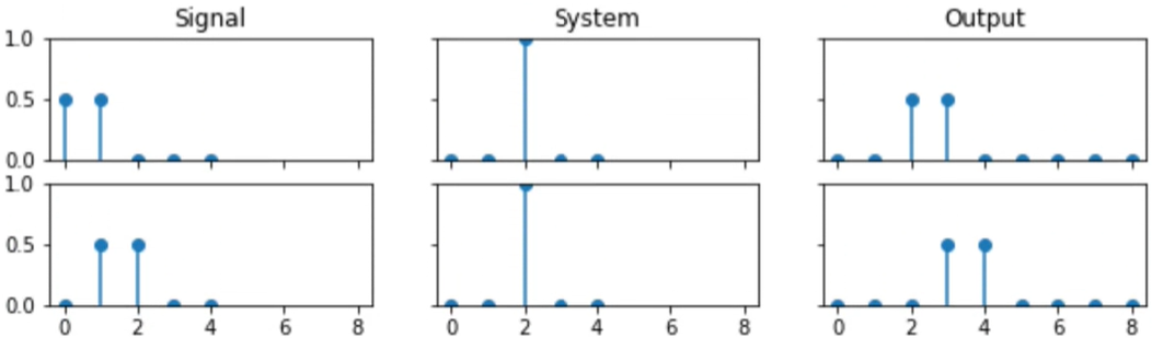
2. Additivity (decompose)
   

   

   : Separately process simple signals and add results together
3. Shift invariance
   

   

   : Shift a signal across (e.g. delay by one unit)

Implement an impulse response by hand:

• Signal = [1.0, 0.75, 0.5, 0.75, 1.0]
• System = [0.0, 1.0, 0.75, 0.5, 0.25]
  • Decompose:
    • input = [0.0, 0.0, 0.0, 0.0, 0.0]
    • input = [0.0, 1.0, 0.0, 0.0, 0.0]
    • input = [0.0, 0.0, 0.75, 0.0, 0.0]
    • input = [0.0, 0.0, 0.0, 0.5, 0.0]
    • input = [0.0, 0.0, 0.0, 0.0, 0.25]
  • Scale:
    • output = [0.0, 0.0, 0.0, 0.0, 0.0]
    • output = [1.0, 0.75, 0.5, 0.75, 1.0]
    • output = [0.75, 0.5625, 0.375, 0.5625, 0.75]
    • output = [0.5, 0.375, 0.25, 0.375, 0.5]
    • output = [0.25, 0.1875, 0.125, 0.1875, 0.25]
  • Shift:
    • output = [0.0, 0.0, 0.0, 0.0, 0.0]
    • output = [0.0, 1.0, 0.75, 0.5, 0.75, 1.0] // delay by one unit
    • output = [0.0, 0.0, 0.75, 0.5625, 0.375, 0.5625, 0.75] // delay by two units
    • output = [0.0, 0.0, 0.0, 0.5, 0.375, 0.25, 0.375, 0.5] // delay by three units
    • output = [0.0, 0.0, 0.0, 0.0, 0.25, 0.1875, 0.125, 0.1875, 0.25] // delay by four units
  • Synthesise (add the components back together):
    • output (result) = [0.0, 1.0, 1.5, 1.5625, 1.75, 2.0, 1.25, 0.6875, 0.25]

Implement in Python:

import numpy as np

def convolve(signal, system):
    rst = np.zeros(len(signal) + len(system) - 1)
    for sig_idx in range(len(signal)):
        sygval = signal[sig_idx]
        for sys_idx in range(len(system)):
            sysval = system[sys_idx]
            scaled = sygval * sysval
            out_idx = sig_idx + sys_idx
            rst[out_idx] += scaled
    return rst

A simple scalar example of audio processing:

• Amplitude is on the y-axis.
• Time is on the x-axis.

Normalisation in audio signals allows us to adjust the volume (amplitude) of the entire signal.

• We can change the size of the amplitude in a proportionate way.

Normalisation in audio signals is a bit simpler than statistical normalisation. It involves two phases: analysis and scaling.

1. Analysis phase
   : In this phase, the signal is analysed to find the peak, or the loudest sample. This is essentially a peak-finding algorithm that identifies the highest amplitude in the waveform.
2. Scaling phase
   : Once the peak is found, the algorithm calculates how much gain can be applied to the entire signal without causing clipping (distortion). This gain is then applied uniformly to the entire signal.

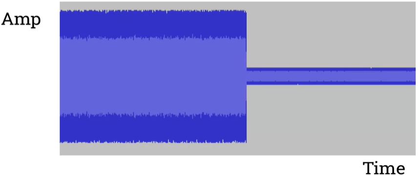
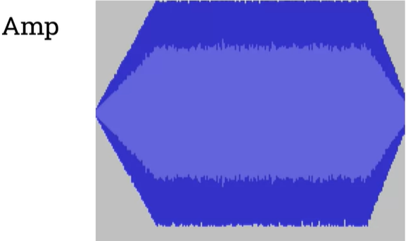
Linear ramps: fading in and out

• Fade in
  : It starts with the scalar zero so that mutes the signal and then gradually as we go through that range, we're increasing the scalar up to one when it hits which would make no change to the signal so effectively turns back to the original signal.
• Fade out
  : It starts out with a high scalar at the beginning of the array of numbers that we're going to process. As the effect, as we've iterated over the numbers in the array, we will reduce that scalar down to zero and then obviously that would sound like the signal getting quieter.