Welcome To Sora Park

The meaning of 'bio-inspired' is as follows:

• Looking at the algorithms and functions in the natural world and thinking there must be something we can use computationally here

According to Wikipedia, bio-inspired computing (short for biologically inspired computing) is a field of study which seeks to solve computer science problems models of biology.

• It relates to connectionism, social behaviour, and emergence.

Within computer science, bio-inspired computing relates to artificial intelligence (AI) and machine learning (ML).

Bio-inspired computation has emerged as one of the most studied branches of AI during the last decades, according to the referece:

• Del Ser, Javier, et al. "Bio-inspired computation: Where we stand and what's next." Swarm and Evolutionary Computation 48 (2019): 220-250.

Brief overview of bio-inspired computing:

• 1950s: Cybernetics
  • "the science of control and communication, in the animal and the machine" - Weiner, 1948
  • "Co-ordination, regulation and control will be its themes, for these are of the greatest biological and practical interest" - Ashby, 1961
• 1960s: Connectionism (neural networks)
  • "The perceptron is a minimally constrained 'nerve net' consisting of logically simplified neural elements, which has been shown to be capable of learning to discriminate and to recognise perceptual patterns" - F. Rosenblatt, 'Perceptron Simulation Experiments,' in Proceedings of the IRE, vol. 48, no. 3, pp. 301-309, March 1960, doi: 10.1109/JRPROC.1960.287598
• 1970s: Genetic algorithms
  • The algorithms were introduced in the US by John Holland at University of Michigan
• 1980s: Artificial life
• 1990s: Onwards and upwards!

Genetic algorithms (GAs) are a type of search algorithm inspired by natural selection. They mimic the process of evolution to find optimal solutions to problems:

• GAs are probabilistic search procedures designed to work on large spaces involving states that can be represented by strings. A space is defined as the space of possible solutions to a problem.
  • Probabilistic search: selection and breeding
  • States: phenotype
  • Strings: genotype

The complete set of genetic material, including all chromosomes, is called a genome.

• The genotype encodes the range of characteristics of the individual DNA (the set of genes in genome).
  • DNA is passed from one generation to the next: heredity
• The phenotype is the actual individual that manifests in the world.

Genotype is set at birth, determined by the DNA inherited from the parents. It's fixed at conception. Phenotype is influenced by both genotype and environment. While genotype provides the blueprint, the environment plays a role in shaping the phenotype. For example, even with a genotype for tallness, nutrition can affect how tall someone becomes.

• Nature vs. Nurture:
  • DNA = Nature
  • Environment = Nurture, defining where in these ranges the characteristics actually fall

The environment plays a crucial role in shaping evolution. It exerts selective pressure on phenotypes, favouring those that are better suited to survive and reproduce.

• These successful phenotypes, with their underlying genotypes, are more likely to be passed on to future generations (heredity).

GAs are inspired by the principles of Darwinian evolution. In GAs, we simulate a population of individuals with varying traits (analogous to phenotypes):

1. Popluation and Variation
   : We start with a population of candidate solutions, each representing a potential answer to the problem. Each solution has its own unique set of characteristics (like genes in an organism).
2. Selection
   : We then select solutions that perform well based on a defined fitness function (similar to how successful phenotypes survive in nature).
3. Reproduction
   : These 'fit' solutions are then used to create new solutions (like breeding in evolution). Techniques like crossover (combining characteristics) and mutation (introducing variations) are used to mimic the processes of inheritance and random genetic changes.

Advantages of GAs:

1. Finding optimal solutions
   : A key advantage of GAs is their ability to locate both local and global maxima (points of highest fitness) within a given search space. This makes them superior to older 'hill-climbing' algorithms that can get stuck at local maxima.
2. Exploring combinations
   : GAs go beyond simply testing individual components. They employ a technique called hyperplane sampling. This essentially means they evaluate various different combinations of these components, mimicking how different genes interact in an organism. This allows GAs to explore a broader range of potential solutions and potentially discover more optimal combinations.

How GAs work:

• Selection
  : Imagine a roulett wheel where each slice represents a member of the population. The size of a slice is determined by a 'fitness function' that evaluates how well that member solves the problem.
  • The fitter a member, the larger its slice, giving it a higher chance of being selected for reproduction. This mimics how natural selection favours organisms better suited to their environment.
• Hyperplane sampling and schemata
  : GAs don't just evaluate individual components of a solution, like bricks in a wall. They can also test different combinations of these components (like building different wall structures).
  • This allows them to find better overall solutions by exploring how different components work together. The schema theorem is a complex concept that supports this ability of GAs.
• Parallelism
  : GAs can leverage parallelism to speed up the search process. There are two main types:
  
  • Implicit parallelism: This uses the population model itself to explore multiple solutions simulaneously. Imagine pairs competing in a tournament, with the winners progressing to the next round.
    → In implicit parallelism, you can only evaluate pairings of individuals in sequence, once at a time.
  • Computational parallelism: If you have a computer with multiple cores, you can use them to evaluate several combinations of individuals at the same time, significantly speeding up the search.
    → In computational parallelism, you can evaluate several combinations of individuals at the same time, depending on how many cores you have on your processor.

Fairness in game playing AI: six key dimensions

1. Perceptual fairness
   : Do both competitors perceive the game environment in the same way? This refers to the information they receive about the game (the same input space).
2. Motoric fairness
   : Do both competitors have the same capabilities to take actions within the game (the same output space)? This includes limitations or advantages in movement, availablr options, or control schemes.
3. Historic fairness
   : Did both AI system have the same amount of time and data for training? This ensures a level playing field by avoiding an advantage for systems with more extensive training data.
4. Knowledge fairness
   : Do both competitors have access to the same in-game knowledge? This refers to understanding the game's rules, objectives, and potentially strategies if applicable.
5. Computational fairness
   : Do both AI systems have the same processing power for decision-making? This ensures neither system has a significant advantage in terms of computational speed or resources.
6. Common-sense fairness
   : Do both AI have access to the same background knowledge beyond the specific game? This includes common-sense reasoning that could influence gameplay decisions.

Isaac Asimov's three laws of robotics:

1. The First Law
   : A robot may not injure a human being or, through inaction, allow a human being to come to harm.
   → This law prioritises human safety above all else.
2. The Second Law
   : A robot must obey the orders given it by human beings except where such orders would conflict with the First Law.
   → Robots are programmed to follow human instructions, but not at the expense of harming humans.
3. The Third Law
   : A robot must protect its own existence as long as such protection does not conflict with the First or Second Law.
   → Robots are given a basic instinct for self-preservation, but overridden by the higher priorities of protecting humans and following orders.

In the field of reinforcement learning, the action policy is a mapping between states and actions, denoted by the Greek letter 'π' (pi). This means that the policy, given state s, will recommend taking action a: π(s) → a.

• State: s
• Action: a
• Next state: s'

A Markov Decision Process is a way of formalising a stochastic sequential decision problem.

• State transitions: P(s' | s, a)
• Reward function: R(s, a, s')

Formalising is basically expressing something in a clear and mathematical way. It can then be used to build algorithms and a stochastic sequential decision problem. Stochastic means it has a probabilistic element. It is sarcastic because it might go to other states probabilistically based on what the current state is.

Unlike a one-time decision, an optimal policy in reinforcement learning considers the long-term reward. It aims to maximise the total reward accumulated over a sequence of actions, even if some rewards come much later.

Bellman equation(ish) defining the value of a given action in a given state based on future reward.

The value of action a in state s is the reward for s + max possible future reward for states s at time t, increasingly discounted by gamma (γ), discount factor, raised to the power of t.

• Gamma (γ) is less than 1.
  • Assuming γ=0.5, then γ squared would be 0.25. So we're only taking a quart in a quarter of the reward. We're not confident of what's going to happen in the future, so we're going to take a little bit of the reward that comes in the future.

Note that the probability of state transitions are not included here.

What are the future states and rewards?

• The state transition matrix describes how the environment reacts to the chosen actions (how the state will change over time based on the chosen actions). It tells us the probability of reaching different states after taking specific actions in the current state.
• The action policy, on the other hand, guides the decision-making. It takes the current state as input and recommends which action to take. This recommendation can be based on maximising immediate reward, long-term reward, or other criteria depending on the specific policy.

In reinforcement learning, creating an optimal action policy often requires complete knowledge of the environment. This includes knowing the transition matrix (all possible state transitions based on actions) and the rewards associated with each transition.

However, in most real-world scenarios, this information is incomplete. Q-learning is a technique that addresses this challenge. It focuses on learning a Q-value function, which estimates the expected future reward for taking a specific action in a particular state.

• The goal of Q-learning is to find the optimal Q-function (Q)*, which tells us the best action to take in any given state to maximise future rewards.

There are various methods to do Q-learning, but most of them don't work for real problems. The one that works here is to approximate the value function using a deep network called Deep Q Network (DQN).

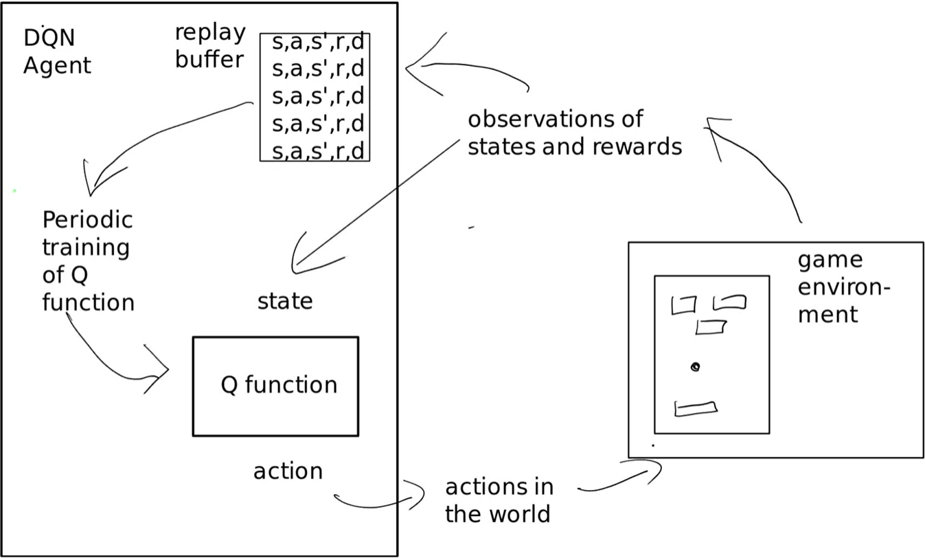
DQN agent architecture

• An agent is an entity that can observe and act autonomously.
  • We need an agent architecture that solves two problems: no state transition matrix and no action policy.

We explore the game and make observations of the form: s, a, s', r, and done.

• s = state now
• a = action taken
• s' = next state
• r = reward
• done = true/false is the game finished?

For DQN, this is the 'replay buffer'. Over time, the agent fills up a large replay buffer. The example for one state, s1, and the three actions, a1/a2/a3 is as follows:

1. s1, a1 → s2, r1, d0
2. s1, a2 → s3, r2, d0
3. s1, a3 → s4, r3, d1

The epsilon greedy exploration is the method that the agent uses to fill up the replay buffer. The acting policy is a simple and effective method for balancing exploration and exploitation by estimating the highest rewards.

• Epsilon-greedy works by introducing a probability (epsilon, ε) of taking a random action instead of the one with the highest estimated Q-value. This encourages exploration and helps the agent discover potentially better actions it might not have encountered yet.

The DQN agent

• Knows about the states and rewards
• Acts in the game world by taking actions
• Makes observations of what is happening in the game
• Replay buffer consists of many observations of the actions taken by the agent in the game world and the results of those actions

In Deep Q-Networks (DQN), a crucial part of the training process is the loss function. This function helps the network learn by measuring the difference between its predictions and the desired outcome.

• The theta (Θ) is the weight in the network.
• Θ￣ is the old version of the network.

To train the network, we use a technique called experience replay. We store past experiences (state, action, reward, next state) in a replay buffer (D). During training, we uniformly sample a mini-batch of these experiences, denoted by U(D), to create a training set. This training set feeds the network and helps it learn from various past experiences.

Assignable or not

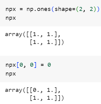
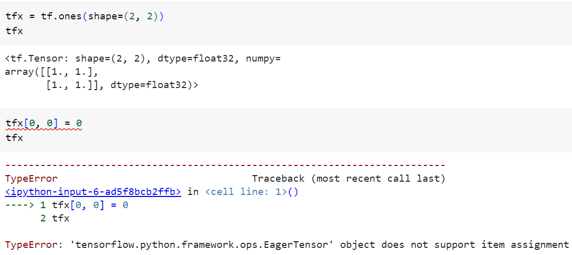
While NumPy arrays are flexible and can be changed (mutable), TensorFlow tensors are fixed (immutable). This means that it is possible to directly modify the values of NumPy arrays, but changing the values of TensorFlow tensors after their creation is not allowed.

For example, the following NumPy array allows itself to be assigned:

In contrast, a TensorFlow tensor cannot be revised as follows:

To update TensorFlow tensors, the tf.Variable class can be used.

Gradient Computation Capabilities

NumPy can't retrieve the gradient of any differentiable expression for any of its inputs. To apply some computation to one or several input tensors and retrieve the gradient of the result with respect to the inputs, just open a GradientTape scope as below:

When dealing with a constant tensor, it needs to be explicitly marked for tracking by calling watch() on it. This is because storing the information required to compute the gradient of anything with respect to anything would be too expensive to do preemptively. The following example utilises watch() to avoid wasting resources, ensuring that the GradientTape knows what to monitor:

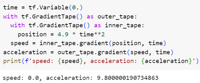
The GradientTape is capable of computing second-order gradients (the gradient of a gradient).

• The gradient of the position of an object with regard to time is the speed of that object.
• The second-order gradient is its acceleration.

Here is an example below: