Welcome To Sora Park

Data representations for neural networks

1. Scalars (rank-0 tensors)
   e.g. np.array(2)
2. Vectors (rank-1 tensors or 1D tensor)
   e.g. np.array([2, 3])
3. Matrices (rank-2 tensors or 2D tensor)
   e.g. np.array([[2, 3], [4, 5]])
4. Rank-3 (3D tensor)
   e.g. np.array([[[2, 3, 4], [5, 6, 7]], [[8, 9, 10], [11, 12, 13]], [[14, 15, 16], [17, 18, 19]]])
          features: 2, width: 3, samples: 1

Tensors are a generalisation of matrices to an arbitrary number of dimensions (a dimension is often called an axis).

Ranks are the number of axes of a tensor.

Tensor operations

• Build a model by stacking Dense layers on top of each other
  
  • Hidden layer: tensorflow.keras.layers.Dense(512, activation="relu")
    
    • This function is as follows: relu(dot(input, W) + b)
    • dot is a dot product between the input tensor and a tensor named W
    • + is an addition between the resulting matrix and a vector b
    • "relu" stands for "rectified linear unit", and relu(x) is equivalent to max(x, 0)
    • "relu" activation is usually used in the hidden layer, especially in the first layer
    • The number of units (neurons), 512 in this case, should be determined based on the complexity of the data. It should not be random.
  • Output layer: tensorflow.keras.layers.Dense(10, activation="softmax")
    • This last layer is a 10-way softmax classification layer, which means it will return an array of 10 probability scores (summing to 1).
• Make the model ready for training at the compilation step
  • optimizer: The mechanism through which the model will update itself based on the training data it sees, to improve its performance.
  • loss: How the model will be able to measure its performance on the training data, and thus how it will be able to steer itself in the right direction. The purpose of loss functions is to compute the quantity that a model should seek to minimise during training.
  • metrics: This function is used to judge the performance of a model (monitor during training and testing).
• Fit the model to its training data
  
  • epochs
  • batch_size

The three screenshots are excerpts from the code available at https://github.com/we1c0me2s0rapark/UoL-MLNN/blob/main/MNIST.ipynb

In the above case, given the shape of the training data as (60000, 784), the number of gradient updates is calculated as 2345, obtained from ((60000/128) * 5).

Deep neural networks do the input-to-target mapping via a deep sequence of simple data tranformations (layers). This transformation implemented by a layer is parameterised by its weights. Weights are also sometimes called the parameters of a layer.

• Learning means finding a set of values for the weights of all layers in a network.

The network will correctly map the inputs to their associated targets only if the weights are reasonable.

• To control the output of a neural network, we need to be able to measure how far this output is from what we expected. This is the job of the loss function of the network. The loss function is also sometimes called the objective function or cost function.

The loss function takes the predictions of the network and the true target and computes a distance score, capturing how well the network has done.

The fundamental trick in deep learning is to use this score as a feedback signal to adjust the value of the weights a little, in a direction that will lower the loss score. This adjustment is the job of the optimiser, which implements what's called the backpropagation algorithm, which is the central algorithm in deep learning.

With every example the network processes, the weights are adjusted a little in the correct direction, and the loss score decreases. This is the training loop.

헵 규칙 (Hebb rule) 은 최초의 신경망 학습 규칙 중 하나로, 1949년 도널드 헵 (Donald O. Hebb) 이 뇌의 시냅스 변형 메커니즘으로 제안한 이후로 인공 신경망 훈련에 사용되고 있다.

당시 헵이 집필한 'The Organization of Behavior' 책에는 헵 학습으로 알려진 가정 (공리) 이 있다.

세포 A의 축삭이 세포 B를 자극하기에 충분히 가깝고 B를 발화하는 데 반복적 또는 지속적으로 참여할 때, 한쪽 또는 양쪽 세포에 일종의 성장 과정이나 신진대사의 변화가 일어남으로써 B를 발화하는 세포 중 하나로서 A의 효율이 올라간다.

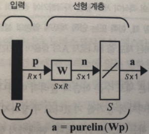
헵 학습 규칙은 다양한 신경망 구조와 결합해서 사용할 수 있다. 예를 들어 선형 연상 메모리 (linear associator) 가 있다.

이는 연상 메모리 (associative memory) 라고 하는 신경망 종류의 한 예로, 연상 메모리의 작업은 프로토타입 입력/출력 벡터의 Q개 쌍을 학습하는 것이다.

$$ \{p_1,t_1\}, \{p_2,t_2\}, ... , \{p_Q,t_Q\} $$

네트워크가 입력 p를 받으면 출력 t를 생성해야 하는데, 입력이 바뀌면 출력도 약간 바뀌어야 한다.

시냅스 양쪽에 있는 두 뉴런이 동시에 활성화되면 시냅스의 강도는 증가하게 될 것이다.

• 위 그림에서 입력 p와 출력 a의 연결 (시냅스) 은 가중치 w이다.

헵의 가정은 양의 p가 양의 a를 생성한다면 w가 증가해야 한다는 것을 의미한다. 수학적 해석은 아래와 같다.

• p는 q번째 입력 벡터의 j번째 요소
• a는 q번째 입력 벡터가 네트워크에 제시될 때 네트워크 출력의 i번째 요소
• 알파는 양의 상수이며, 학습률 (learning rate) 이라고 부름

이 식은 가중치 w의 변화가 시냅스 양쪽의 활성 함수의 곱에 비례한다는 사실을 말해준다.

참고로 이 식에 정의된 헵 규칙은 비지도 학습 (unsupervised learning) 규칙이므로, 목표 출력에 관련된 정보가 필요 없다. 지도 (supervised) 헵 규칙에서는 실제 출력을 목표 출력으로 대체할 수 있다.

이 방법은 알고리즘에게 '네트워크가 현재 하고 있는 것'이 아닌 '네트워크가 해야만 하는 것'을 알려준다.

• t는 q번째 목표 벡터 t의 i번째 요소
• 학습률은 1로 설정

벡터 표기법은 아래와 같다.

$$ W^N=W^O+t_qp_q^T $$

가중치 행렬을 0으로 초기화하고 Q개의 입력/출력 쌍을 한번에 적용하면 아래와 같이 작성할 수 있다.

$$ W=t_1p_1^T+t_2p_2^T+ ... +t_QP_Q^T=\sum_{q=1}^{Q}t_qp_q^T $$

이 식은 행렬 방식으로 표현될 수 있다.

$$ W=\begin{bmatrix}
t_1 & t_2 & ... & t_Q \\
\end{bmatrix}\begin{bmatrix}
p_1^T \\ p_2^T \\ ... \\ p_Q^T
\end{bmatrix}=TP^T $$

여기서

$$ T=\begin{bmatrix}
t_1 & t_2 & ... & t_Q \\
\end{bmatrix}, P=\begin{bmatrix}
p_1 & p_2 & ... & p_Q \\
\end{bmatrix} $$

선형 연상 메모리에 대한 헵 학습의 성능 분석 시 프로토타입 벡터 (p_q) 가 직교하면서 단위 길이를 갖는 정규직교 (orthonormal) 인 경우와 단위 길이를 갖지만 직교하지 않는 경우를 나눠서 살펴볼 수 있다.

1. 정규직교인 경우:
   p_k 가 네트워크 입력이면 네트워크 출력은 다음과 같이 계산된다.
   $$ a=Wp_k=(\sum_{q=1}^{Q}t_qp_q^T)p_k=\sum_{q=1}^{Q}t_q(p_q^Tp_k) $$
   p_q 가 정규직교이기 때문에 다음과 같이 된다.
   $$ (p_q^Tp_k)=1, q=k $$
   $$ (p_q^Tp_k)=0, q!=k $$
   Identity matrix 가 되기 때문에 네트워크 출력은 다음과 같이 간단하게 작성될 수 있다.
   $$ a=Wp_k=t_k $$
2. 단위 길이이지만, 직교가 아닌 경우:
   벡터가 직교하지 않기 때문에 네트워크는 정확한 출력을 생성하지 않을 것이며, 오차의 크기는 프로토타입 입력 패턴 사이에 상관 관계의 크기에 따라 달라진다.
   $$ a=Wp_k=t_k+\sum_{q!=k}^{}t_q(p_q^Tp_k) $$
   우항의 시그마는 오차를 나타낸다.

예제 1) 입력 벡터가 정규직교일 때

$$ p_1=\begin{bmatrix}
0.5 \\ -0.5 \\ 0.5 \\ -0.5
\end{bmatrix}, t_1=\begin{bmatrix}
1 \\ -1
\end{bmatrix}  $$

$$ p_2=\begin{bmatrix}
0.5 \\ 0.5 \\ -0.5 \\ -0.5
\end{bmatrix}, t_2=\begin{bmatrix}
1 \\ 1
\end{bmatrix} $$

가중치 행렬:

$$ W=TP^T=\begin{bmatrix}
1 & 1 \\
-1 & 1 \\
\end{bmatrix}\begin{bmatrix}
0.5 & -0.5 & 0.5 & -0.5 \\
0.5 & 0.5 & -0.5 & -0.5 \\
\end{bmatrix}=\begin{bmatrix}
1 & 0 & 0 & -1 \\
0 & 1 & -1 & 0 \\
\end{bmatrix} $$

각각의 프로토타입 입력에 대한 가중치 행렬 테스트 결과:

$$ Wp_1=\begin{bmatrix}
1 & 0 & 0 & -1 \\
0 & 1 & -1 & 0 \\
\end{bmatrix}\begin{bmatrix}
0.5 \\ -0.5 \\ 0.5 \\ -0.5 \\
\end{bmatrix} =\begin{bmatrix}
1 \\ -1
\end{bmatrix} $$

$$ Wp_2=\begin{bmatrix}
1 & 0 & 0 & -1 \\
0 & 1 & -1 & 0 \\
\end{bmatrix}\begin{bmatrix}
0.5 \\ 0.5 \\ -0.5 \\ -0.5 \\
\end{bmatrix}=\begin{bmatrix}
1 \\ 1
\end{bmatrix} $$

네트워크 출력이 목표와 동일하다는 것을 알 수 있다.

예제 2) 입력 벡터가 직교하지 않을 때

$$ p_1=\begin{bmatrix}
1 \\ -1 \\ -1
\end{bmatrix},
p_2=\begin{bmatrix}
1 \\ 1 \\ -1
\end{bmatrix} $$

두 프로토타입 입력을 정규화하고 희망 출력을 -1과 1로 각각 선택하면 다음과 같다.

$$ p_1=\begin{bmatrix}
0.5774 \\ -0.5774 \\ -0.5774
\end{bmatrix}, t_1=\begin{bmatrix}
-1
\end{bmatrix} $$

$$ p_2=\begin{bmatrix}
0.5774 \\ 0.5774 \\ -0.5774
\end{bmatrix}, t_2=\begin{bmatrix}
1
\end{bmatrix} $$

가중치 행렬:

$$ W=TP^T=\begin{bmatrix}
-1 & 1
\end{bmatrix}\begin{bmatrix}
0.5774 & -0.5774 & -0.5774 \\
0.5774 & 0.5774 & -0.5774 \\
\end{bmatrix}=\begin{bmatrix}
1 & 1.1548 & 0
\end{bmatrix} $$

두 프로토타입 패턴을 가중치 행렬과 곱하면 다음과 같다.

$$ Wp_1=\begin{bmatrix}
0 & 1.1548 & 0
\end{bmatrix}\begin{bmatrix}
0.5774 \\ -0.5774 \\ -0.5774
\end{bmatrix} =\begin{bmatrix}
-0.6668
\end{bmatrix} $$

$$ Wp_2=\begin{bmatrix}
0 & 1.1548 & 0
\end{bmatrix}\begin{bmatrix}
0.5774 \\ 0.5774 \\ -0.5774
\end{bmatrix} =\begin{bmatrix}
0.6668
\end{bmatrix} $$

출력이 목표 출력과 일치하지 않는다.

학습 규칙 (learning rule) 은 네트워크의 가중치와 편향을 변경하는 방법을 의미한다. 학습 규칙은 크게

• 지도 학습 (supervised learning)
• 비지도 학습 (unsupervised learning)
• 강화 학습 (reinforcement learning)

으로 분류할 수 있다.

지도 학습은 훈련 집합 (training set) 과 같은 예시를 학습 규칙에 제공한다.

$$ \{p_1,t_1\}, \{p_2,t_2\}, ... , \{p_Q,t_Q\} $$

p는 네트워크 입력이며, t는 대응되는 정확한 출력 (목표) 이다.

1. 각 입력을 네트워크에 적용해서 네트워크 출력과 목표를 비교한다.
2. 네트워크 출력이 목표에 가까워지도록 학습 규칙을 사용해 네트워크의 가중치와 편향을 조정한다.

지도 학습에서 이진 분류로 결과가 나올 경우 그 출력을 discrete output 이라고 하며, classification problem 이 이에 해당한다. 시간의 흐름에 따라 값을 예측하는 경우 그 출력을 continuous output 이라고 하며, regression problem 이 이에 해당한다.

지도 학습은 훈련 알고리즘 (training algorithm) 에 네트워크 입력에 대한 목표를 제공하지만, 강화 학습은 등급 (또는 점수) 을 부여한다. 등급은 연속적인 입력에 대한 네트워크 성능 척도다. 강화 학습에는 액션에 따른 보상 (reward) 이 주어지며, 보상에 따라 액션을 바꿔가며 더 나은 결과를 유도한다.

비지도 학습은 사용 가능한 목표 출력이 없고, 네트워크 입력에 대한 반응만으로 가중치와 편향을 변경한다. 대부분의 비지도 학습 알고리즘은 군집화 연산을 수행해서 입력 패턴을 한정된 수의 클래스로 범주화 하도록 학습한다.