(w04) Filtering

Signal averaging is a signal processing technique that tries to remove unwanted random disturbances from a signal through the process of averaging.

• Averaging often takes the form of summing a series of signal samples and then dividing that sum by the number of individual samples.

The following equation represents a N-point moving average filter, with input the array x and outputs the averaged array y:

$$ y(n)=\frac{1}{N}\sum_{k=0}^{N-1}x(n-k) $$

 

Implementing in Python:

### 1. Simple example
import numpy as np

values = np.array([3., 9., 3., 4., 5., 2., 1., 7., 9., 1., 3., 5., 4., 9., 0., 4., 2., 8., 9., 7.])
N = 3

averages = np.empty(len(values))
for i in range(1, len(values)-1):
    averages[i] = (values[i-1]+values[i]+values[i+1])/N

# Preserve the edge values
averages[0] = values[0]
averages[len(values)-1] = values[len(values)-1]

### 2. Use numpy.convolve
window = np.ones(3)
window /= sum(window)
averages = np.convolve(values, window, mode='same')

### 3. Use scipy.ndimage.uniform_filter1d
from scipy.ndimage.filters import uniform_filter1d
averages = uniform_filter1d(values, size=3)

 

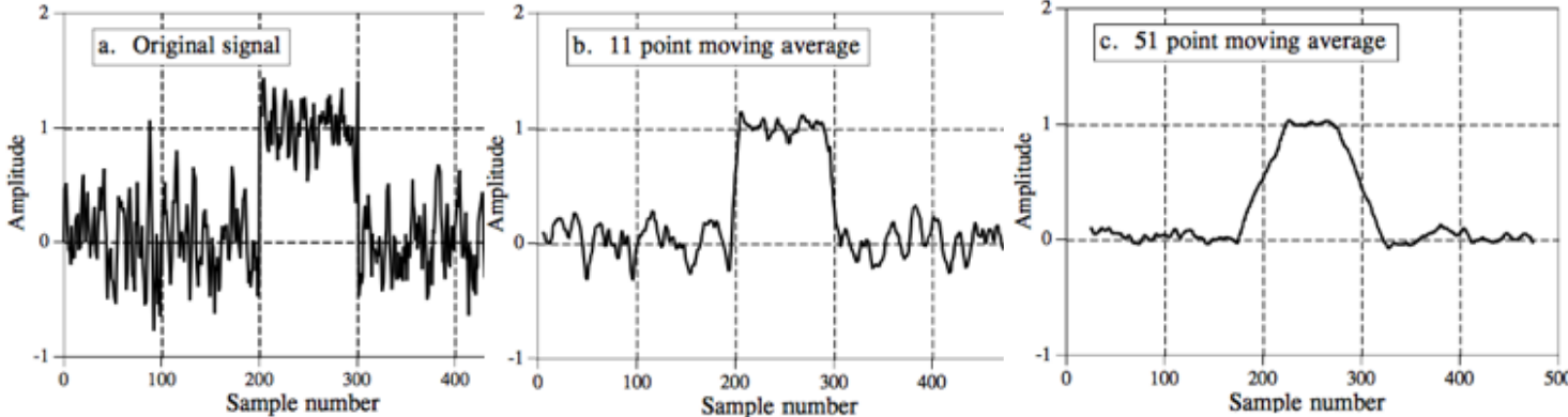
Averaging low-pass filter

In signal processing, the moving average filter can be used as a simple low-pass filter. The moving average filter smooths out a signal, removing the high frequency components from it, and this is what a low-filter does!

 

FIR (Finite Impulse Response) filers

In signal processing, a FIR filer is a filter whose impulse response (or response to any finite length input) is of finite duration, because it settles to zero in finite time. For a general N-tap FIR filter, the nth output is:

$$  y(n)=\sum_{k=0}^{N-1}h(k)x(n-k) $$

$$ h(n)=\frac{1}{N} $$

$$ n=0,1,...,N $$

This fomula has already been used above, since the moving average filter is a kind of FIR filter.

 

Implementing in Python:

import numpy as np
from thinkdsp import SquareSignal, Wave

# suppress scientific notation for small numbers
np.set_printoptions(precision=3, suppress=True)

# The wave to be filtered
from thinkdsp import read_wave
my_sound = read_wave('../Audio/429671__violinsimma__violin-carnatic-phrase-am.wav')
my_sound.make_audio()

# Make a 5-tap FIR filter using the following coefficients: 0.1, 0.2, 0.2, 0.2, 0.1
window = np.array([0.1, 0.2, 0.2, 0.2, 0.1])

# Apply the window to the signal using np.convolve
filtered = np.convolve(my_sound.ys, window, mode='same')
filtered_violin = Wave(filtered, framerate=my_sound.framerate)
filtered_violin.make_audio()

 

LTI (Linear Time Invariant) systems

• It it happens to be a LTI system, we can represent its behaviour as a list of numbers known as an IMPULSE RESPONSE.

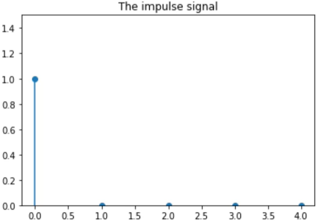
An impulse response is the response of an LTI system to the impulse signal.

• An impulse is one single maximum amplitude sample.

Example of an impulse:

There is one stalk that is reaching up to 0.

Example of an impulse response:

It is a bunch of stalks (a set of numbers).

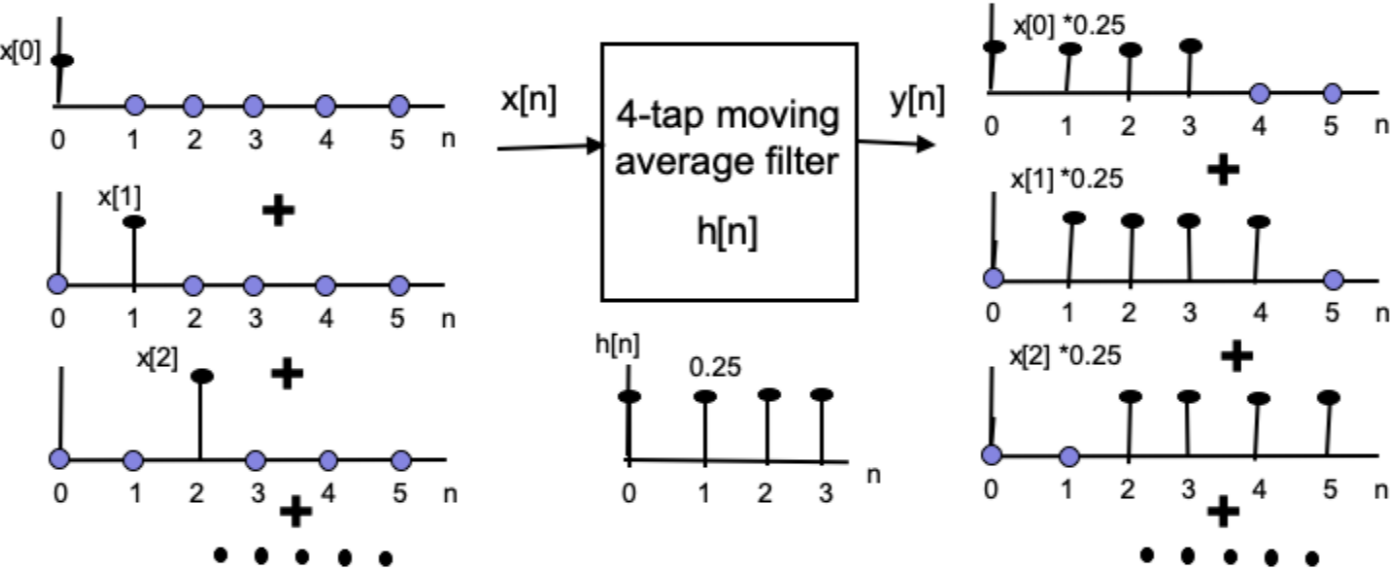
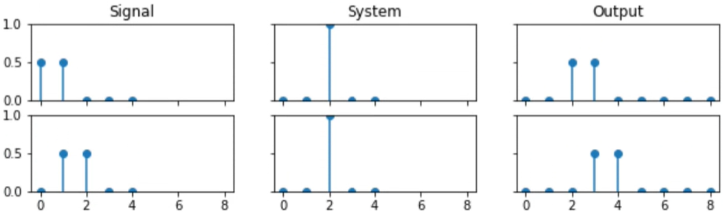
Given an impulse response, we can easily process any signal with that system using convolution.

 

• We can derive the output of a discrete linear system, by adding together the system's response to each input sample separately. This operation is known as convolution.

$$ y[n]=x[n]*h[n]=\sum_{m=0}^{\infty }x[m]h[n-m] $$

※ The convolution operator is indicated by the '*' operator

 

Three characteristics of LTI systems

Linear systems have very specific characteristics which enable us to do the convolution:

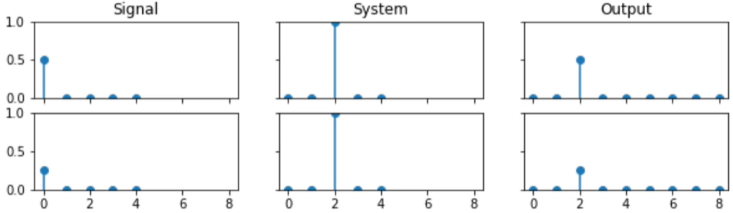
1. Homogeneity (or linear with respect to scale)
   

   

   : Multiply the signal by 0.5 (scale it by 0.5), shove both the signals through the systemsl, and get the outputs
   1) Convolve the signal with the system
   2) Receive the output
   → It doesn't matter if the signal is scaled becuse we know tht it will produce the same scaled output.
2. Additivity (decompose)
   

   

   : Separately process simple signals and add results together
3. Shift invariance
   

   

   : Shift a signal across (e.g. delay by one unit)

Implement an impulse response by hand:

• Signal = [1.0, 0.75, 0.5, 0.75, 1.0]
• System = [0.0, 1.0, 0.75, 0.5, 0.25]
  • Decompose:
    • input = [0.0, 0.0, 0.0, 0.0, 0.0]
    • input = [0.0, 1.0, 0.0, 0.0, 0.0]
    • input = [0.0, 0.0, 0.75, 0.0, 0.0]
    • input = [0.0, 0.0, 0.0, 0.5, 0.0]
    • input = [0.0, 0.0, 0.0, 0.0, 0.25]
  • Scale:
    • output = [0.0, 0.0, 0.0, 0.0, 0.0]
    • output = [1.0, 0.75, 0.5, 0.75, 1.0]
    • output = [0.75, 0.5625, 0.375, 0.5625, 0.75]
    • output = [0.5, 0.375, 0.25, 0.375, 0.5]
    • output = [0.25, 0.1875, 0.125, 0.1875, 0.25]
  • Shift:
    • output = [0.0, 0.0, 0.0, 0.0, 0.0]
    • output = [0.0, 1.0, 0.75, 0.5, 0.75, 1.0] // delay by one unit
    • output = [0.0, 0.0, 0.75, 0.5625, 0.375, 0.5625, 0.75] // delay by two units
    • output = [0.0, 0.0, 0.0, 0.5, 0.375, 0.25, 0.375, 0.5] // delay by three units
    • output = [0.0, 0.0, 0.0, 0.0, 0.25, 0.1875, 0.125, 0.1875, 0.25] // delay by four units
  • Synthesise (add the components back together):
    • output (result) = [0.0, 1.0, 1.5, 1.5625, 1.75, 2.0, 1.25, 0.6875, 0.25]

Implement in Python:

import numpy as np

def convolve(signal, system):
    rst = np.zeros(len(signal) + len(system) - 1)
    for sig_idx in range(len(signal)):
        sygval = signal[sig_idx]
        for sys_idx in range(len(system)):
            sysval = system[sys_idx]
            scaled = sygval * sysval
            out_idx = sig_idx + sys_idx
            rst[out_idx] += scaled
    return rst