Welcome To Sora Park

Assignable or not

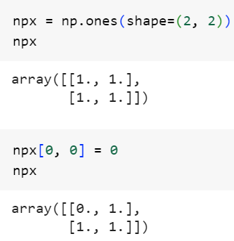
While NumPy arrays are flexible and can be changed (mutable), TensorFlow tensors are fixed (immutable). This means that it is possible to directly modify the values of NumPy arrays, but changing the values of TensorFlow tensors after their creation is not allowed.

For example, the following NumPy array allows itself to be assigned:

In contrast, a TensorFlow tensor cannot be revised as follows:

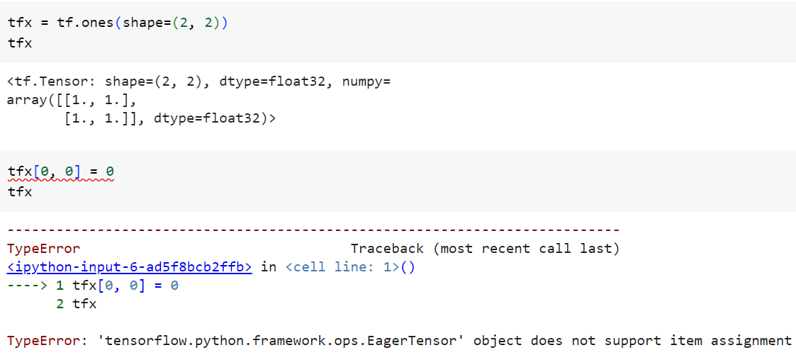
To update TensorFlow tensors, the tf.Variable class can be used.

Gradient Computation Capabilities

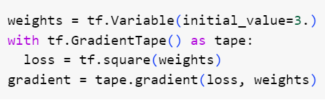
NumPy can't retrieve the gradient of any differentiable expression for any of its inputs. To apply some computation to one or several input tensors and retrieve the gradient of the result with respect to the inputs, just open a GradientTape scope as below:

When dealing with a constant tensor, it needs to be explicitly marked for tracking by calling watch() on it. This is because storing the information required to compute the gradient of anything with respect to anything would be too expensive to do preemptively. The following example utilises watch() to avoid wasting resources, ensuring that the GradientTape knows what to monitor:

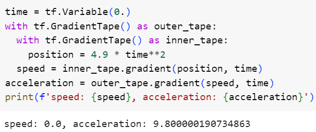
The GradientTape is capable of computing second-order gradients (the gradient of a gradient).

• The gradient of the position of an object with regard to time is the speed of that object.
• The second-order gradient is its acceleration.

Here is an example below:

A least-squares problem is an optimisation problem with no constraints and an objective, which is as follows:

minimise

$$ f_0(x)=\left\|Ax-b \right\|_2^2=\sum_{i=1}^{k}(a_i^Tx-b_i)^2 $$

The objective function is a sum of squares of terms of the form

$$ a_i^Tx-b_i $$

The solution can be reduced to solving a set of linear equations,

$$ f(x)=\left\| Ax-b\right\|_2^2=(A_x-b)^T(Ax-b) $$

$$ =((Ax)^T-b^T)(Ax-b) $$
$$ =x^TA^TAx-b^TAx-x^TA^Tb+b^Tb $$

If x is a global minimum of the objective function, then its gradient is the zero vector.

$$ \triangledown f(x)=(\frac{\partial f}{\partial x_1},...,\frac{\partial f}{\partial x_n}) $$

The gradients are:

$$ \triangledown(x^TA^TAx)=2A^TAx, \triangledown(b^TAx)=A^Tb, \triangledown(x^TA^Tb)=A^Tb $$

Calculate these gradients with respect to

$$ x_1,...,x_n $$

Thus, the gradient of the objective function is

$$ \triangledown f(x)=2A^TAx-A^Tb-A^Tb=2A^TAx-2A^Tb $$

To find the least squares solution, we can solve

$$ \triangledown f(x)=0 $$

Or equivalently

$$ A^TAx=A^Tb $$

So we have the analytical solution:

$$ x=(A^TA)^{-1}A^Tb $$

To recognise an optimisation problem as a least-squares problem, we only need to verify that the objective is a quadratic function.