Welcome To Sora Park

A least-squares problem is an optimisation problem with no constraints and an objective, which is as follows:

minimise

$$ f_0(x)=\left\|Ax-b \right\|_2^2=\sum_{i=1}^{k}(a_i^Tx-b_i)^2 $$

The objective function is a sum of squares of terms of the form

$$ a_i^Tx-b_i $$

The solution can be reduced to solving a set of linear equations,

$$ f(x)=\left\| Ax-b\right\|_2^2=(A_x-b)^T(Ax-b) $$

$$ =((Ax)^T-b^T)(Ax-b) $$
$$ =x^TA^TAx-b^TAx-x^TA^Tb+b^Tb $$

If x is a global minimum of the objective function, then its gradient is the zero vector.

$$ \triangledown f(x)=(\frac{\partial f}{\partial x_1},...,\frac{\partial f}{\partial x_n}) $$

The gradients are:

$$ \triangledown(x^TA^TAx)=2A^TAx, \triangledown(b^TAx)=A^Tb, \triangledown(x^TA^Tb)=A^Tb $$

Calculate these gradients with respect to

$$ x_1,...,x_n $$

Thus, the gradient of the objective function is

$$ \triangledown f(x)=2A^TAx-A^Tb-A^Tb=2A^TAx-2A^Tb $$

To find the least squares solution, we can solve

$$ \triangledown f(x)=0 $$

Or equivalently

$$ A^TAx=A^Tb $$

So we have the analytical solution:

$$ x=(A^TA)^{-1}A^Tb $$

To recognise an optimisation problem as a least-squares problem, we only need to verify that the objective is a quadratic function.

The form is as follows:

minimise $$  f_0(x) $$

subject to $$  f_1(x)\leq b_i, i=1,...,m $$

The optimisation variable of the problem is the following vector:

$$ x=(x_1,...,x_n) $$

The objective function is

$$ f_0:R^n\to R $$

The constraint functions are

$$ f_i:R^n\to R $$

The constrants are

$$ b_1,...,b_m $$

Note that the constrants are the limits or bounds for the constraints.

The smallest objective value among all vectors that satisfy the constraints is the optimal or solution of the problem:

$$ x^* $$

For example,

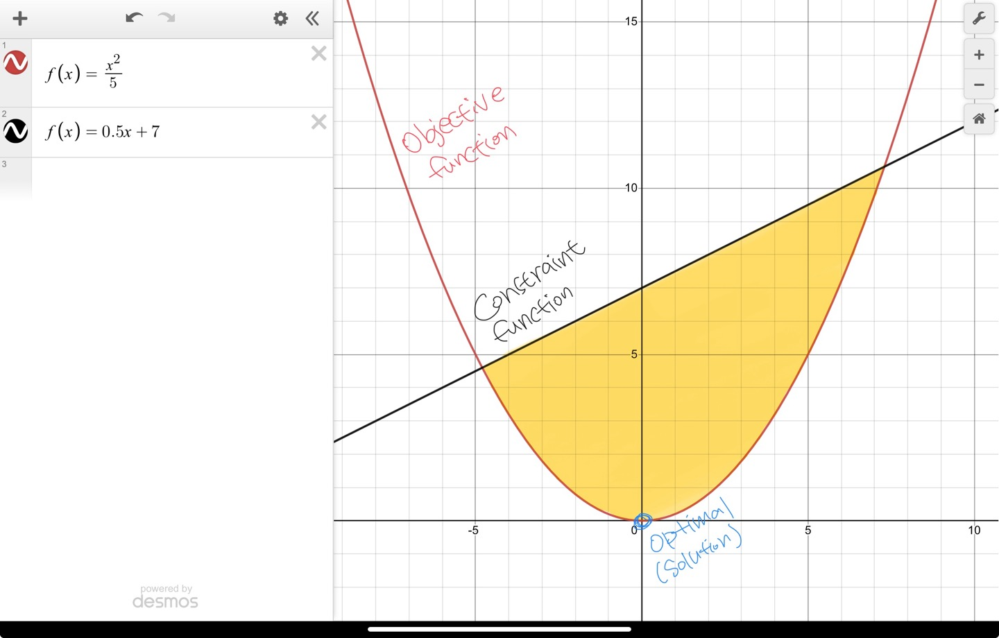
The following convex function (red coloured quadratic function) is

$$ f(x)=2^2/5 $$

The constraint function (black coloured linear function) is

$$ f(x)=0.5x+7 $$

The feasible area is coloured in yellow:

$$ f_1(z) \leq b_1,...,f_m(z) \leq b_m $$

for any z, we have

$$ f_1(z) \leq f_0(x^*) $$

Deep neural networks do the input-to-target mapping via a deep sequence of simple data tranformations (layers). This transformation implemented by a layer is parameterised by its weights. Weights are also sometimes called the parameters of a layer.

• Learning means finding a set of values for the weights of all layers in a network.

The network will correctly map the inputs to their associated targets only if the weights are reasonable.

• To control the output of a neural network, we need to be able to measure how far this output is from what we expected. This is the job of the loss function of the network. The loss function is also sometimes called the objective function or cost function.

The loss function takes the predictions of the network and the true target and computes a distance score, capturing how well the network has done.

The fundamental trick in deep learning is to use this score as a feedback signal to adjust the value of the weights a little, in a direction that will lower the loss score. This adjustment is the job of the optimiser, which implements what's called the backpropagation algorithm, which is the central algorithm in deep learning.

With every example the network processes, the weights are adjusted a little in the correct direction, and the loss score decreases. This is the training loop.

단위 벡터 (unit vector) 는 크기가 1인 벡터를 말한다. 그리고 어떤 벡터를 단위 벡터로 만드는 것을 정규화 (normalisation) 라고 한다.

3차원 벡터를 아래와 같이 정의하면

$$ u=(x,y,z) $$

이 벡터의 크기는 다음과 같이 계산할 수 있다.

$$ \left\| u\right\|=\sqrt{x^2+y^2+z^2} $$

이 벡터를 정규화해서 단위 벡터로 만드는 방법은 벡터의 크기로 각 성분을 나누면 된다.

$$ \hat{u}=\frac{u}{\left\| u\right\|}=
(\frac{x}{\left\| u\right\|}, \frac{y}{\left\| u\right\|}, \frac{z}{\left\| u\right\|})=
(\frac{x}{\sqrt{x^2+y^2+z^2}}, \frac{y}{\sqrt{x^2+y^2+z^2}}, \frac{z}{\sqrt{x^2+y^2+z^2}}) $$

정규화 한 벡터의 크기를 구하면

$$ \left\| \hat{u}\right\|=
\sqrt{(\frac{x}{\sqrt{x^2+y^2+z^2}})^2, (\frac{y}{\sqrt{x^2+y^2+z^2}})^2, (\frac{z}{\sqrt{x^2+y^2+z^2}})^2}=
\sqrt{\frac{x^2+y^2+z^2}{x^2+y^2+z^2}}  $$

이 단위 벡터의 크기는 1이 되는 것을 알 수 있다.