A Fourier Transform (FT) is an integral transform that takes a function as input and outputs another function that describes the extent to which various frequencies are present in the original function.
Discrete Fourier Transform (DFT)
- Since the real world deals with discrete data (samples), the DFT is a crucial tool. It's the discrete version of the FT, specifically designed to analyse finite sequences of data points like those captured by computers.
- The DFT transforms these samples into a complex-valued function of frequency called the Discrete-Time Fourier Transform (DTFT).
DFT converts a finite sequence of equally-spaced samples of a function into a same-length sequence of equally-spaced samples of the discrete-time Fourier transform (DTFT), which is a complex-valued function of frequency.
Discrete Cosine Transform (DCT)
- The DCT is closely related to the DFT. While DFT uses both sines and cosines (complex functions), DCT focuses solely on cosine functions. This makes DCT computationally simpler and often preferred for tasks where the data has even symmetry (like audio signals).
DCT expresses a finite sequence of data points in terms of a sum of cosine functions oscillating at different frequencies.
Fast Fourier Transform (FFT)
- The DFT is powerful, but calculating it directly can be computationally expensive for large datasets. This is where the Fast Fourier Transform (FFT) comes in. It's a highly optimized algorithm specifically designed to compute the DFT efficiently, especially when the data length is a power of 2 (like 16, 32, 64 etc.).
- The FFT is not a theoretical transform. It is just a fast algorithm to implement the transforms when N=2^k.
FFT is an algorithm that computes the Discrete Fourier Transform (DFT) of a sequence, or its inverse (IDFT). IDFT is a Fourier series, using the DTFT samples as coefficients of complex sinusoids at the corresponding DTFT frequencies.
The first step is to move from simple synthesis to complex synthesis.
What's wrong with the DCT?
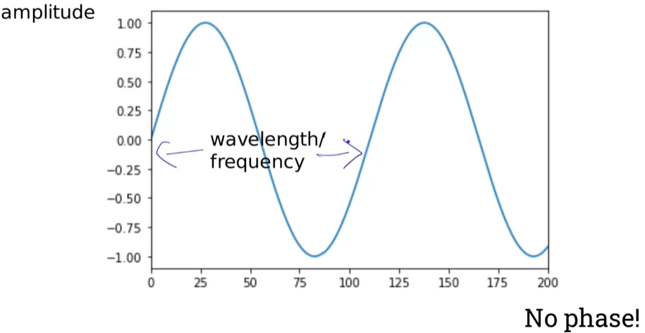
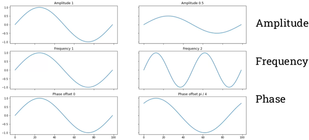
The properties of sinusoids (sine waves): frequency, phase, and amplitude
We need a way to store phase and amplitude in the same place. That is called a complex numbers.
- A complex number is basically two numbers stuck together.
- Think of them as a way of storing phase and amplitude in one place, with associated mathematics to work with the complex numbers similarly to how we work with 'simple' numbers.
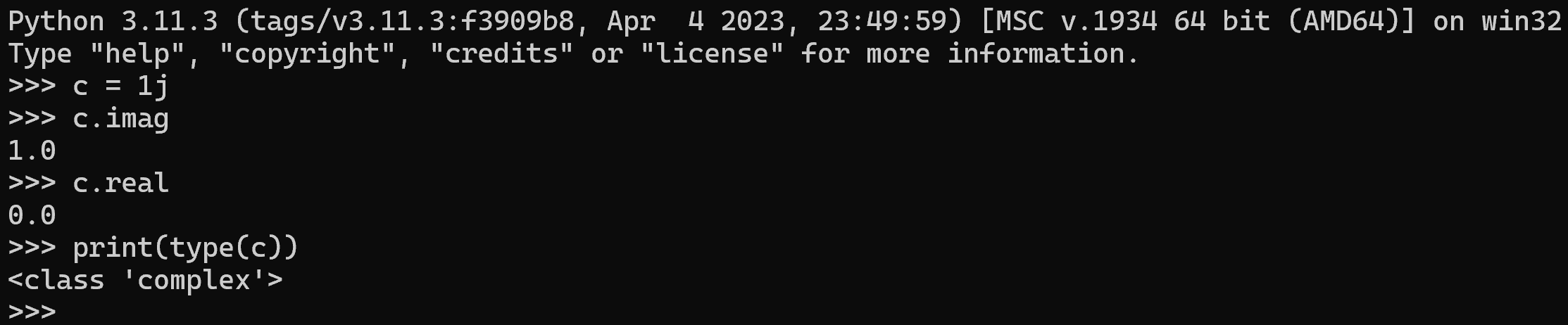
→ Complex numbers have a real and an imaginary part (two numbers).
- Think of them as a way of storing phase and amplitude in one place, with associated mathematics to work with the complex numbers similarly to how we work with 'simple' numbers.
Complex numbers in Python:
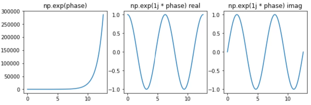
We need a way to computer waveforms from complex numbers: the exponential function
- numpy.exp(x) is the exponential function, or
- e^x (where e is Euler's number: approximately 2.718281)
→ numpy.exp(1j * x) converts x into a complex number then does exp!
Simple synthesis:
def synthesise_simple(amps, fs, ts):
    args = np.outer(ts, fs)
    M = np.cos(np.pi*2 * args)
    ys = np.dot(M, amps)
    return ys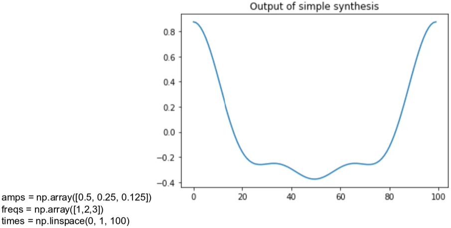
Complex synthesis:
def synthesise_complex(amps, fs, ts):
    args = np.outer(ts, fs)
    M = np.exp(1j * np.pi*2 * args) # Swap out from np.cos(np.pi*2 * args)
    ys = np.dot(M, amps)
    return ys
The complex analysis problem:
- Given a signal and a set of frequencies, how can we find the amplitude and phase of each frequency component?
Simple analysis with numpy.linalg.solve and the DCT:
def analyse_simple(ys, fs, ts):
    args = np.outer(ts, fs)
    M = np.cos(np.pi*2 * args)
    amps = np.linalg.solve(M, ys)
    return amps

# More constrained version
def dct_iv(ys):
    N = len(ys)
    ts = (0.5 + np.arange(N)) / N
    fs = (0.5 + np.arange(N)) / 2
    args = np.outer(ts, fs)
    M = np.cos(np.pi*2 * args)
    amps = np.dot(M, ys) / (N / 2)
    return amps
Complex analysis with np.linalg.solve:
def analyse_complex(ys, fs, ts):
    args = np.outer(ts, fs)
    M = np.exp(1k * np.pi*2 * args)
    amps = np.linalg.solve(M, ys)
    return amps
def analyse_nearly_dft(ys, fs, ts):
    N = len(fs)
    args = np.outer(ts, fs)
    M = np.exp(1j * np.pi*2 * args)
    amps = M.conj().transpose().dot(ys) / N # Swap out from 'amps = np.linalg.solve(M, ys)
    return amps
Final steps for the actual DFT:
# Calculate the frequency and time matrix
def synthesis_matrix(N):
    ts = np.arange(N) / N
    fs = np.arange(N)
    args = np.outer(ts, fs)
    M = np.exp(1j * np.pi*2 * args)
    return M

# Transform
def dft(ys):
    N = len(ys)
    M = synthesis_matrix(N)
    amps = M.conj().transpose().dot(ys) # No more '/ N'!
    return amps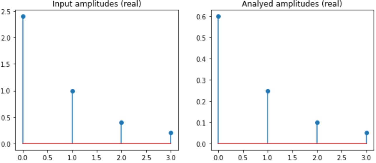
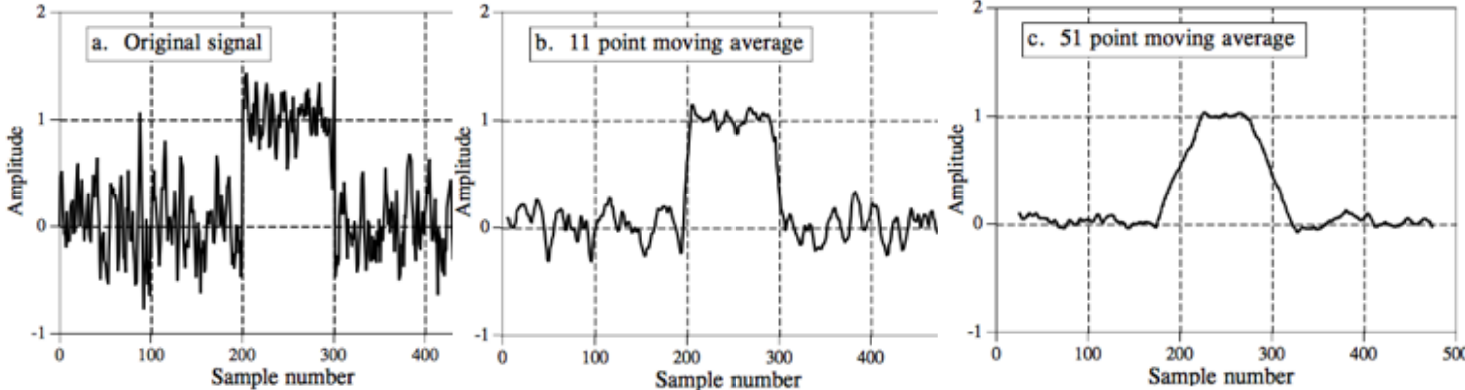
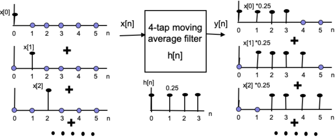
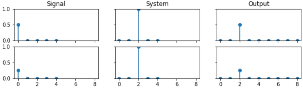
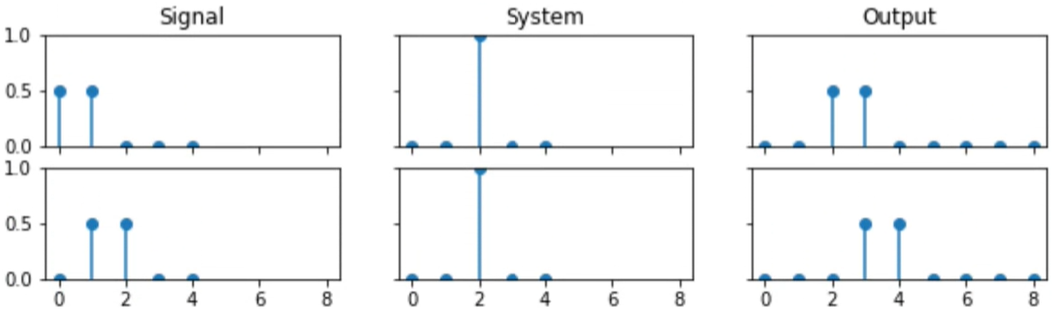
Fast convolution with the DFT

- Convolving signals in the time domain is equivalent to multiplying their Fourier transforms in frequency domain.
The inverse DFT
def idft(ys):
    N = len(ys)
    M = synthesis_matrix(N)
    amps = M.dot(ys) / N
    return amps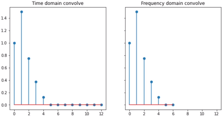
'IntelligentSignalProcessing' 카테고리의 다른 글
| (w10) Offline ASR (Automatic Speech Recognition) system (0) | 2024.06.11 |
|---|---|
| (w04) Filtering (0) | 2024.05.01 |
| (w03) Audio processing (0) | 2024.04.26 |
| (w01) Digitising audio signals (0) | 2024.04.11 |
| (w01) Audio fundamentals (0) | 2024.04.11 |